Python Figure Visualization

Scientific Figures for Research Papers

@seokhyun choung|January 2026

0

Seminar Background

Figures are more than half of paper writing. Good figures elevate your research impact.

Seeing is believing - figures are critical for visual communication
Adopt an automation mindset with open-sourcing culture
Origin/Excel: Intuitive but hard to automate, not suitable for LLM era

0.1

Figure Gallery: Multi-Panel Figures

Complex figures combining multiple data types and visualizations

TEM + XAS + Conversion + Radar plot

Conversion + Raman + XPS + Correlations

0.2

Figure Gallery: Computational Figures

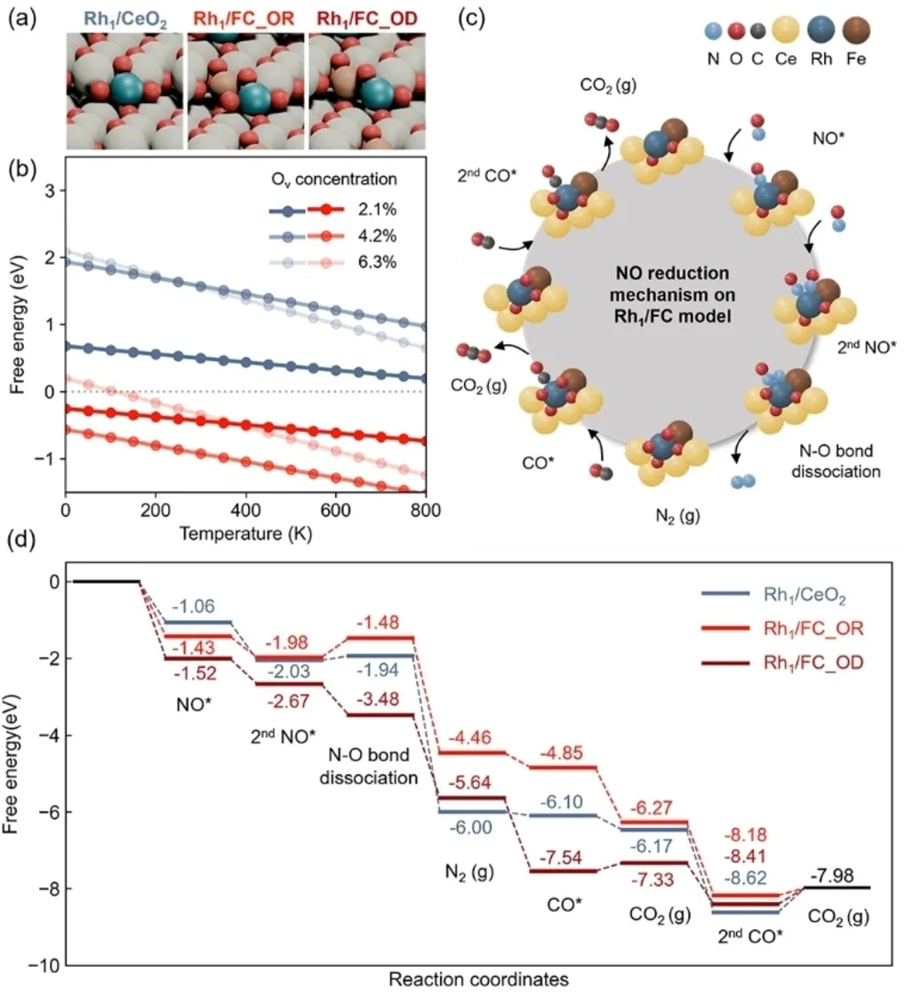
DFT calculations, MD simulations, and ML results

3D vacancy map + violin plot + time series + bar chart

Atomic structures + phase diagram + energy profile

0.3

Figure Gallery: Specialized Plots

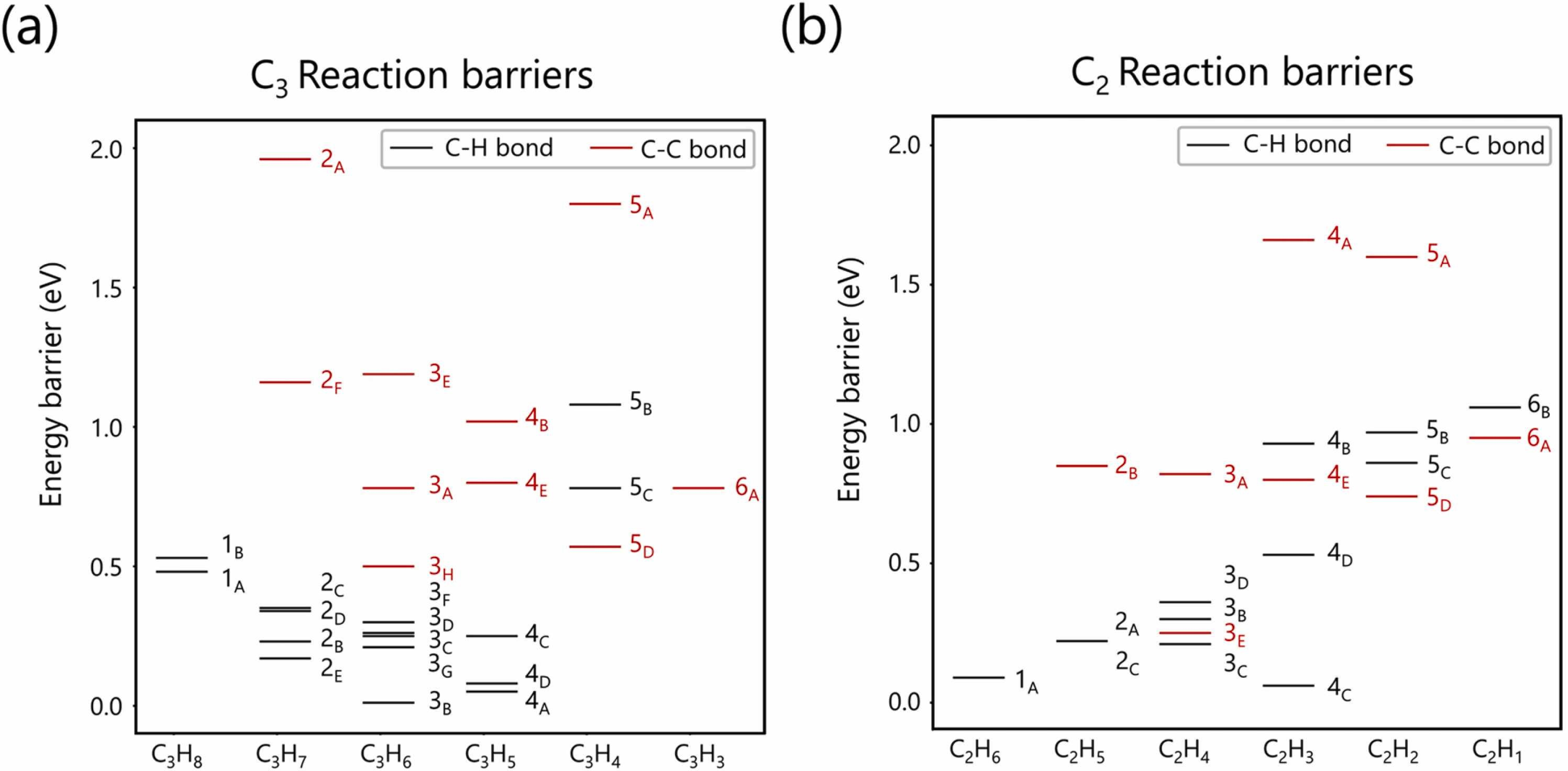
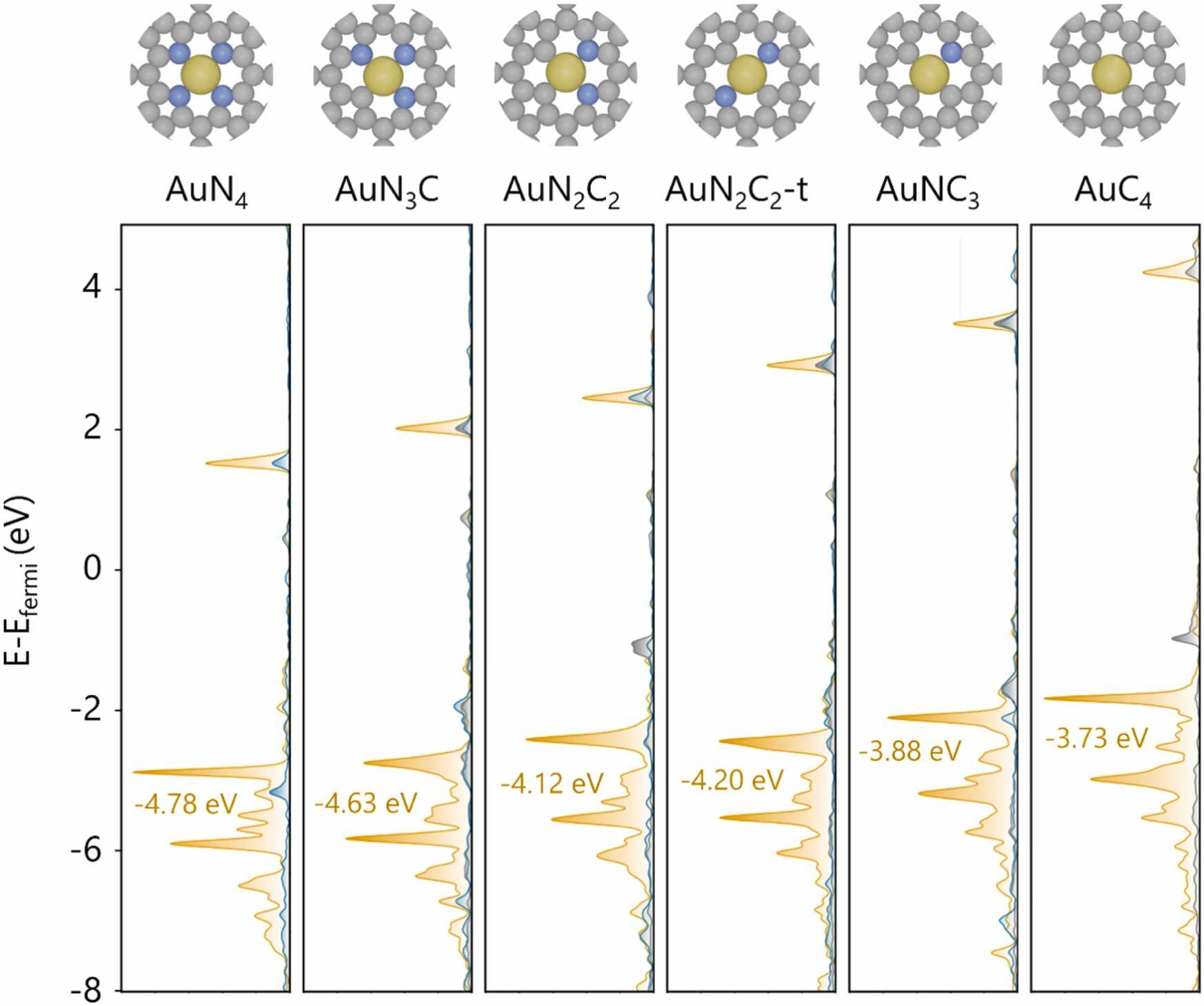
C-H/C-C bond breaking barriers

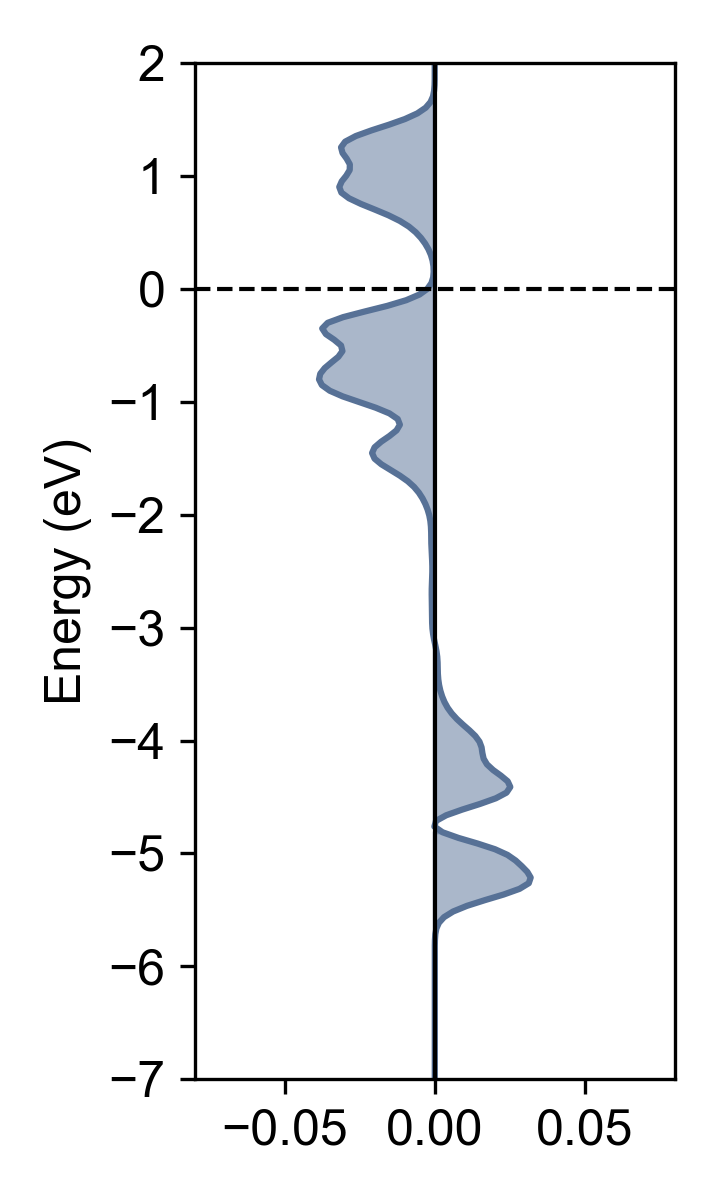
Density of States (DOS)

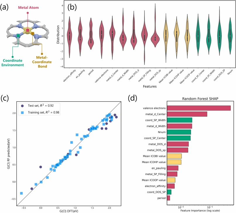
ML: Parity plot + Violin + SHAP

COHP bonding analysis

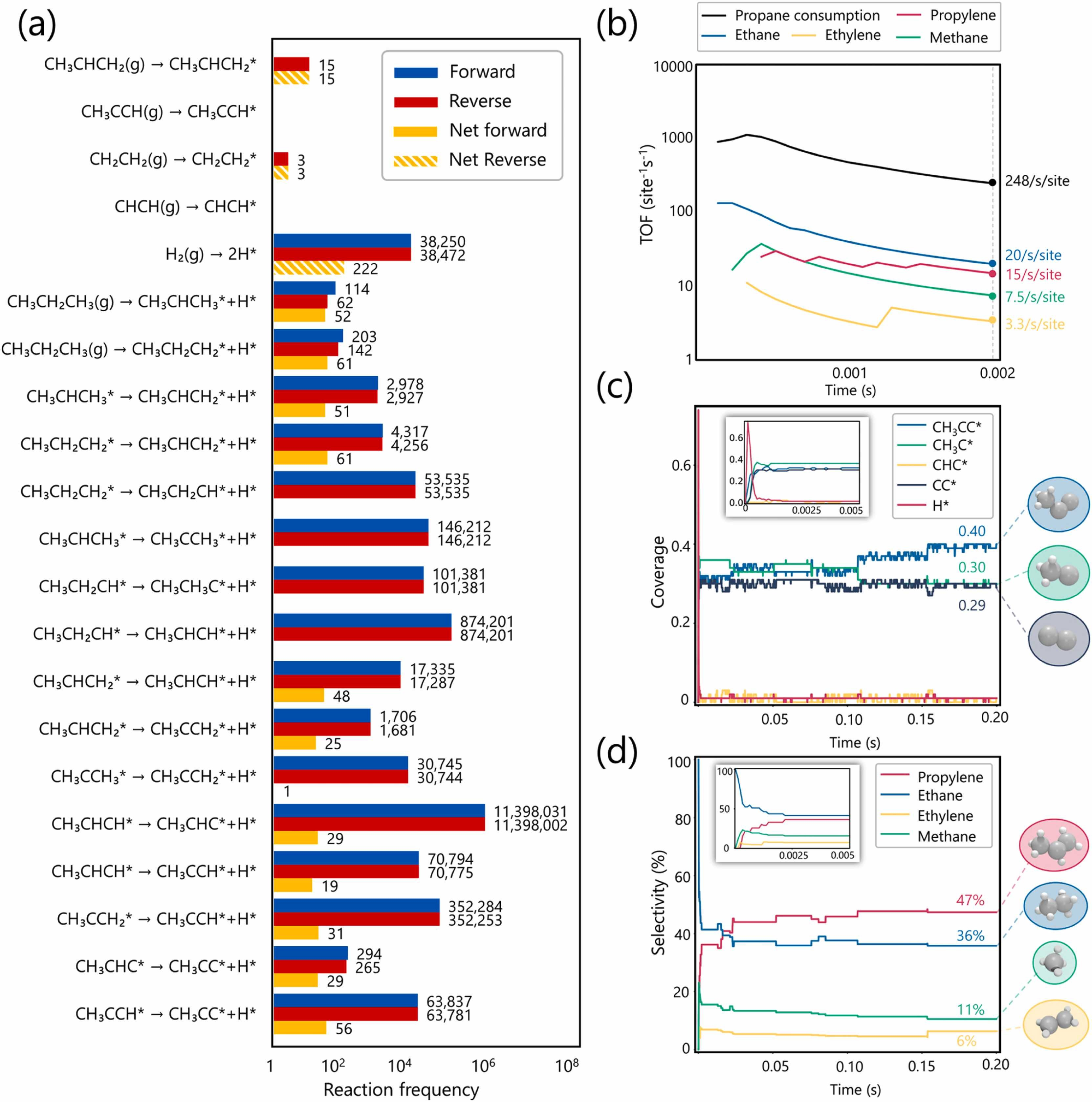
Microkinetic: TOF + Coverage + Selectivity

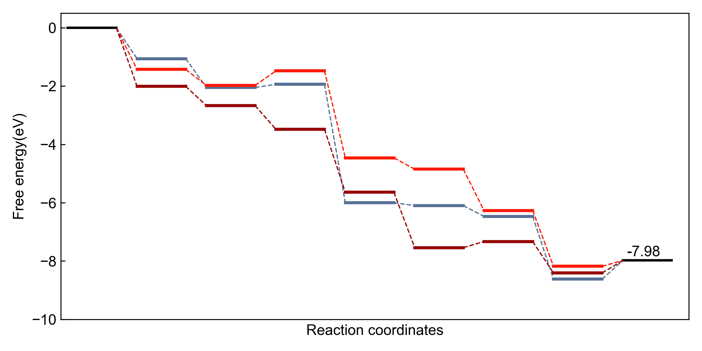
Reaction coordinate diagram

1

Why Python?

Automation in the LLM Era

1.1

Why Python & What Makes Good Figures?

Why Python?

Automation: if you do it twice, automate it
LLM era enables full automation
Code-based = reproducible & version-controlled
Focus on research, not repetitive tasks

Good Figures Have...

Aesthetic: color harmony, visual appeal
Intelligence: clear research message
Convention: follow field standards
Principles: one color/shape = one meaning

->

Python + LLM = Efficient, reproducible, beautiful figures

1.2

Example: Energy Diagrams & Electrochemistry

Structures + thermodynamics + energy diagram

Reaction coordinate with multiple pathways

Polarization curves (j vs E)

Volcano plot + mechanism + charge density

2

Python Basics

Setup, Matplotlib, Data Handling

2.1

Environment Setup & Imports

Conda Setup

# Create environment
conda create -n mpl python=3.9
conda activate mpl

# Install packages
conda install matplotlib pandas numpy
pip install ase  # optional

Basic Imports

import matplotlib.pyplot as plt
import numpy as np
import pandas as pd

# For custom fonts
import matplotlib.font_manager as fm

IDE Options

VSCode / Cursor (AI-powered)
Google Colab

Key Libraries

matplotlib: plotting
numpy: arrays
pandas: data I/O

2.2

Figure, Axes & Plot Types

fig, ax Pattern (recommended)

fig, ax = plt.subplots(figsize=(8, 6))
ax.plot(x, y, color='blue', lw=2)

# Multiple subplots
fig, axes = plt.subplots(2, 3)
axes[0, 0].plot(x, y)

Plot Types

# Line plot
ax.plot(x, y, 'b-', label='data')

# Scatter plot
ax.scatter(x, y, s=50, alpha=0.7)

# Fill between
ax.fill_between(x, y1, y2, alpha=0.3)

Always use fig, ax pattern. Scatter for raw data, lines for continuous/processed data.

2.3

Labels, Limits, Legend & Saving

Formatting

# Labels and limits
ax.set_xlabel('Temperature (C)')
ax.set_ylabel('Conversion (%)')
ax.set_xlim(0, 100)
ax.set_ylim(0, 100)

# Legend
ax.legend(loc='upper right')

Saving

# Always use tight_layout first!
plt.tight_layout()

# Save with options
plt.savefig('fig.png', dpi=300,
            bbox_inches='tight')
plt.savefig('fig.svg')  # vector

SVG format best for publications (vector, scalable)

dpi=300 minimum for print quality

Reverse axis for XPS: ax.set_xlim(x.max(), x.min())

2.4

Data Handling: NumPy & Pandas

NumPy Arrays

# Vectorized operations (fast!)
data = np.array([1, 2, 3, 4, 5])
squared = data**2  # all at once

# Create arrays
x = np.linspace(0, 10, 100)
x = np.arange(0, 10, 0.1)
y = np.sin(x)

Pandas for Excel/CSV

df = pd.read_excel('data.xlsx',
                   sheet_name='Sheet1')

# Select columns
x = df.iloc[:, 0]  # by position
y = df['col_name']  # by name

# Clean data
df = df.dropna()  # remove NaN

Use .values to convert pandas Series to numpy array for plotting.

3

LLM Acceleration

AI-Powered Figure Generation

3.1

LLM Tools & System Prompt

💬

Chatbots

Good for ideation, quick snippets

✎

Cursor

Fine-tuning, in-editor AI

💻

Claude Code

Full automation, vibe coding

🚀

Copilot

Code completion

# System prompt for consistent figures
fs = 12  # font size
font_props = fm.FontProperties(family='Arial', size=fs)
colors = ['#77AEB3', '#E5885D', '#C7C4B5', '#A1C2DE', '#B4944B']
os.makedirs('./output', exist_ok=True)

3.2

Helper Functions & Complete Example

def format_axis(ax, xlabel, ylabel):
    ax.set_xlabel(xlabel, fontproperties=font_props)
    ax.set_ylabel(ylabel, fontproperties=font_props)

def save_plot(filename):
    plt.tight_layout()
    plt.savefig(f'./output/{filename}', dpi=300, bbox_inches='tight')

# Complete example
x = np.linspace(0, 10, 100)
fig, ax = plt.subplots(figsize=(8, 6))
ax.plot(x, np.sin(x), 'b-', lw=2, label='sin(x)')
ax.plot(x, np.cos(x), 'r--', lw=2, label='cos(x)')
ax.fill_between(x, np.sin(x), np.cos(x), where=(np.sin(x)>np.cos(x)), alpha=0.3)
format_axis(ax, 'X values', 'Y values')
ax.legend()
save_plot('trig.svg')

3.3

Key Takeaways

1Use fig, ax pattern

2Set labels with units

3tight_layout() before save

4bbox_inches='tight'

5Use alpha for layers

6SVG for publications

1

NumPy + Pandas

Arrays for speed, DataFrames for Excel/CSV

2

Matplotlib

fig/ax pattern, consistent styling, proper saving

3

LLM Tools

Cursor for fine-tuning, Claude Code for automation

Beautiful Figures Tell Stories

Automate, Iterate, Perfect

Good figures take practice

Automation saves time for creativity

LLMs are your coding partners

Keep coding. Keep visualizing. Keep publishing.