Python 그래프 시각화

연구 논문을 위한 과학적 그래프 작성

@seokhyun choung|2026년 1월

0

세미나 배경

그래프는 논문 작성의 절반 이상입니다. 좋은 그래프는 연구의 영향력을 높입니다.

백문이 불여일견 - 그래프는 시각적 커뮤니케이션의 핵심
오픈소스 문화와 함께 자동화 마인드셋 채택
Origin/Excel: 직관적이지만 자동화 어려움, LLM 시대에 부적합

0.1

그래프 갤러리: 다중 패널 그래프

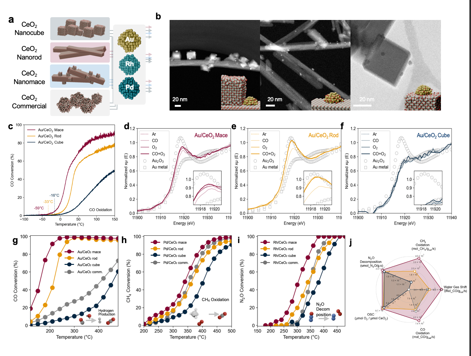
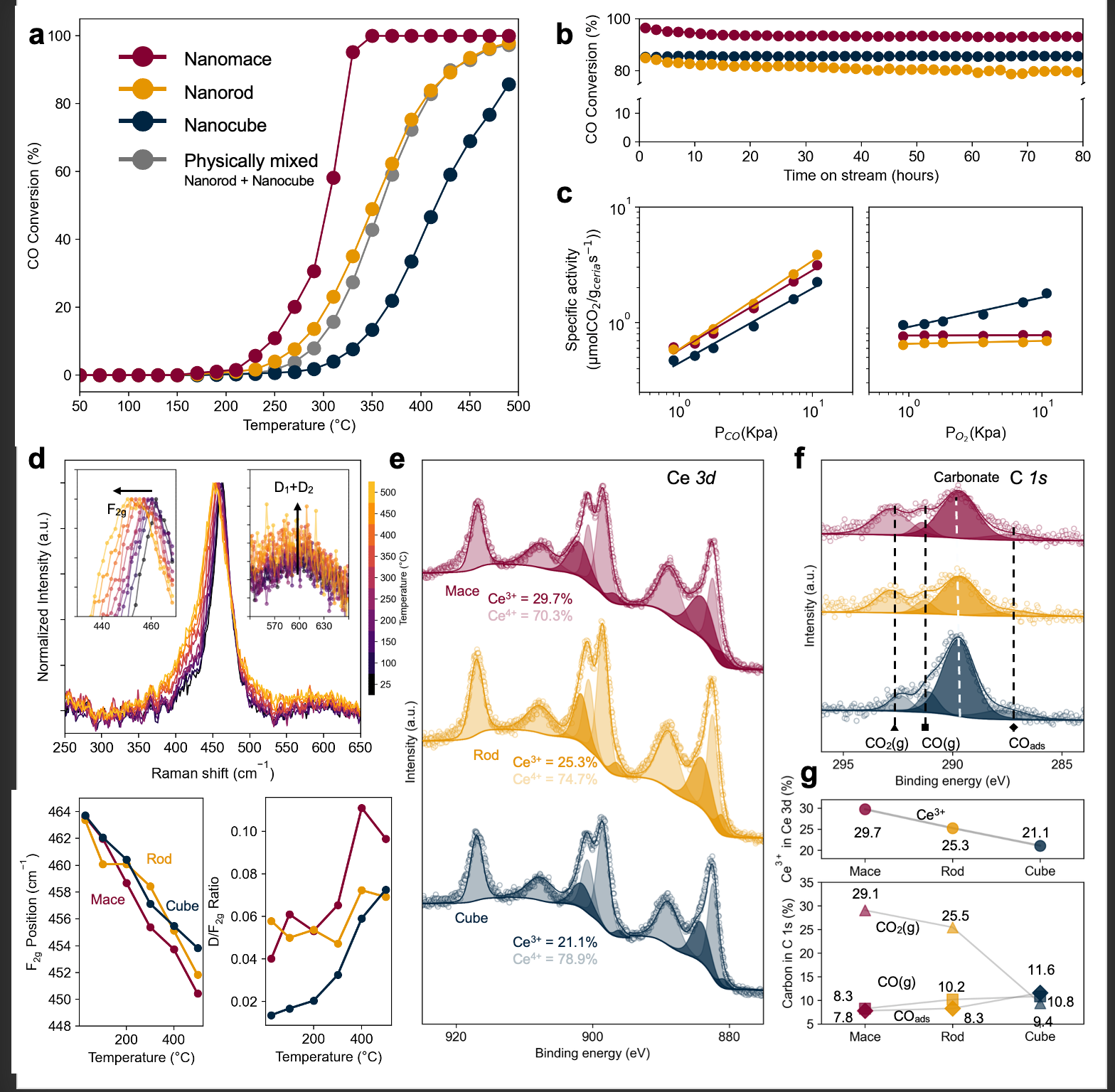
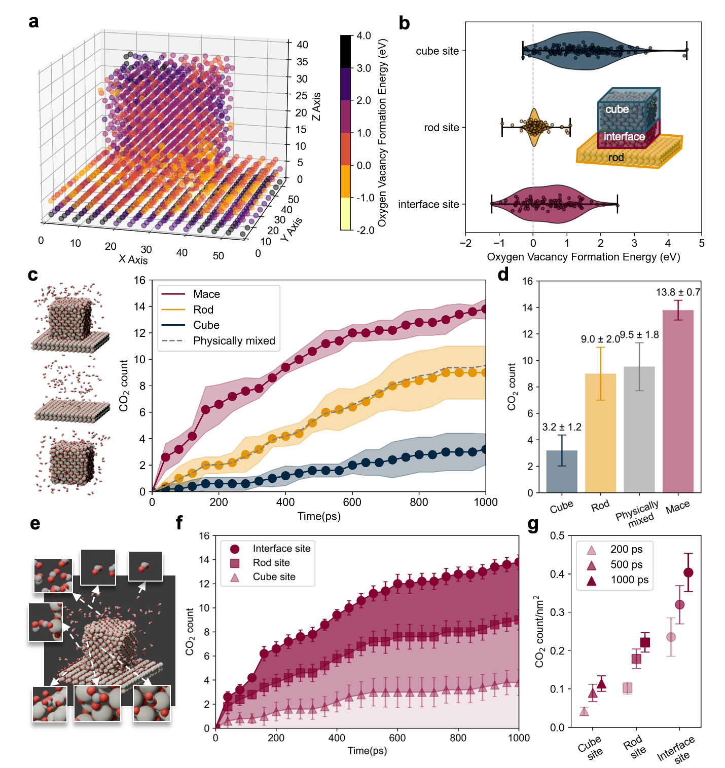
여러 데이터 유형과 시각화를 결합한 복잡한 그래프

TEM + XAS + 전환율 + 레이더 플롯

전환율 + Raman + XPS + 상관관계

0.2

그래프 갤러리: 계산 그래프

DFT 계산, MD 시뮬레이션, ML 결과

3D 빈자리 맵 + 바이올린 플롯 + 시계열 + 막대 차트

원자 구조 + 상다이어그램 + 에너지 프로파일

0.3

그래프 갤러리: 특수 플롯

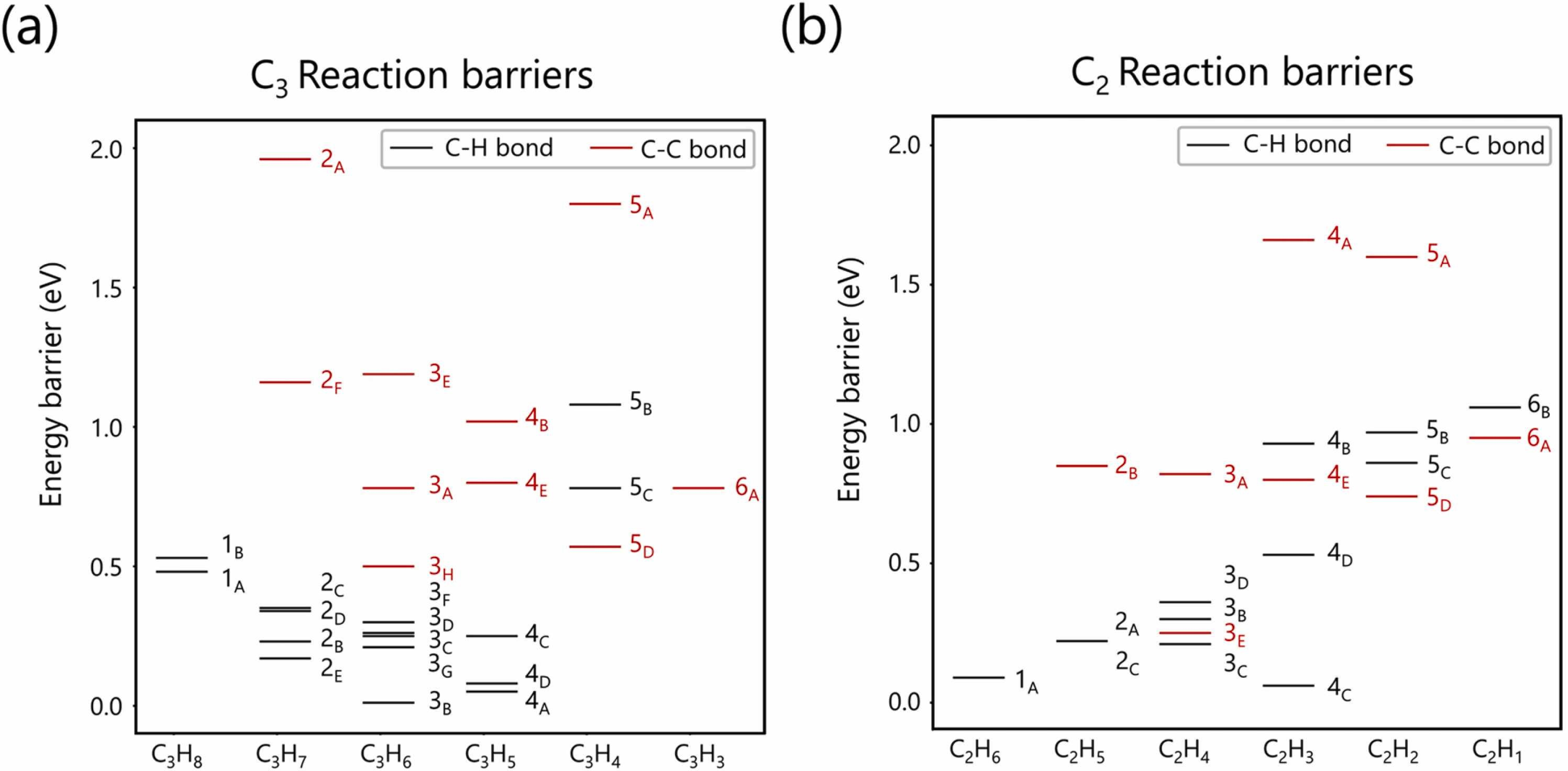
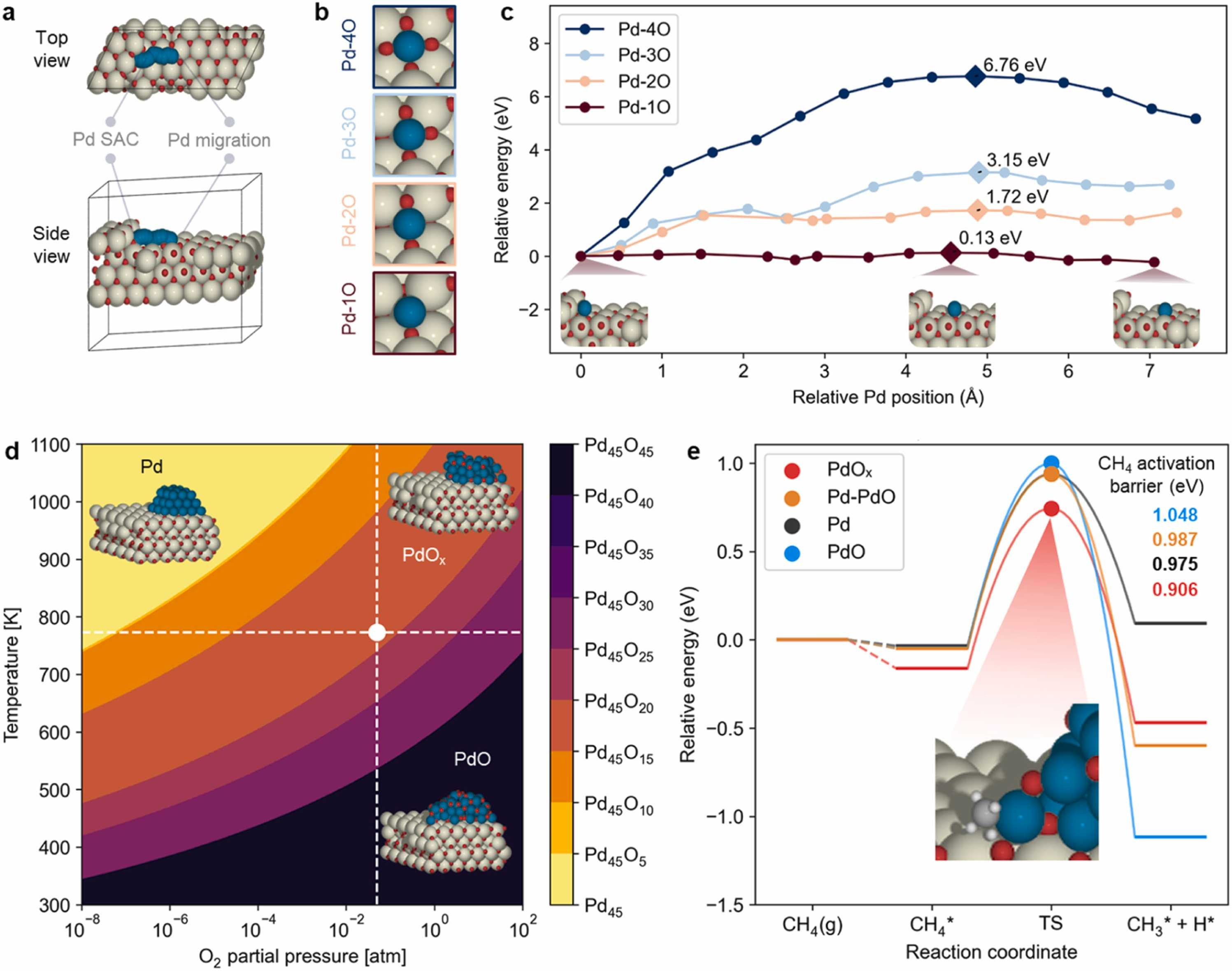
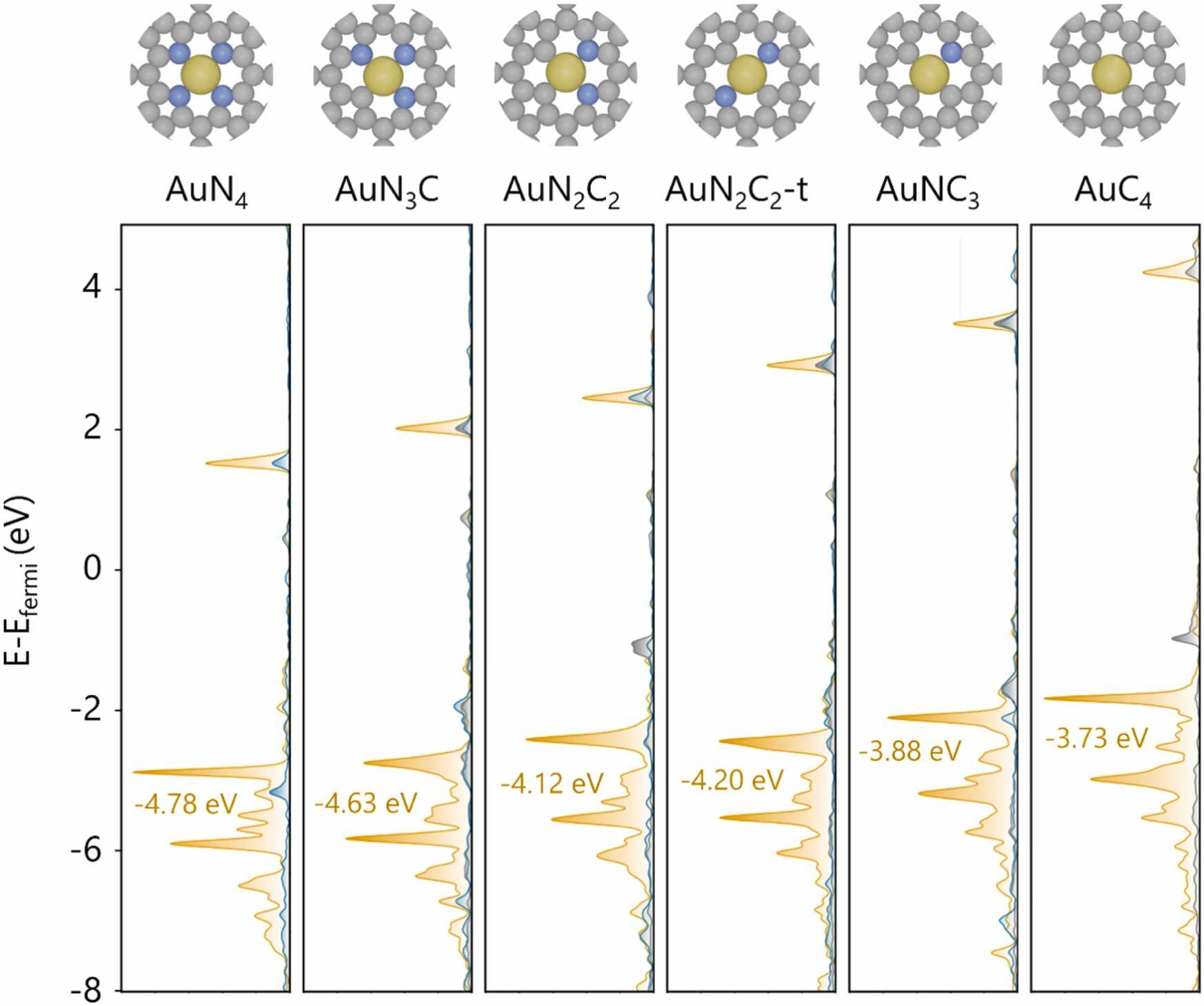
C-H/C-C 결합 끊김 장벽

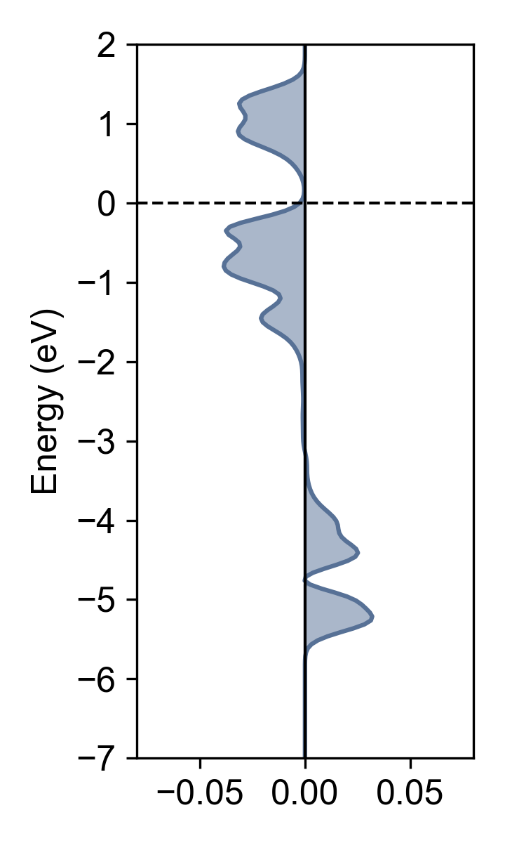
상태 밀도 (DOS)

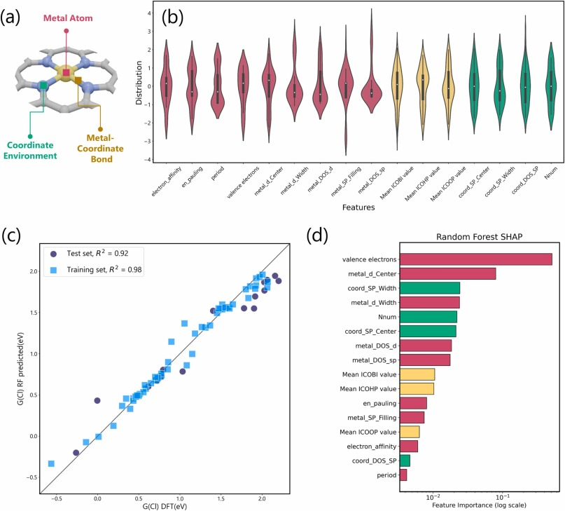
ML: 패리티 플롯 + 바이올린 + SHAP

COHP 결합 분석

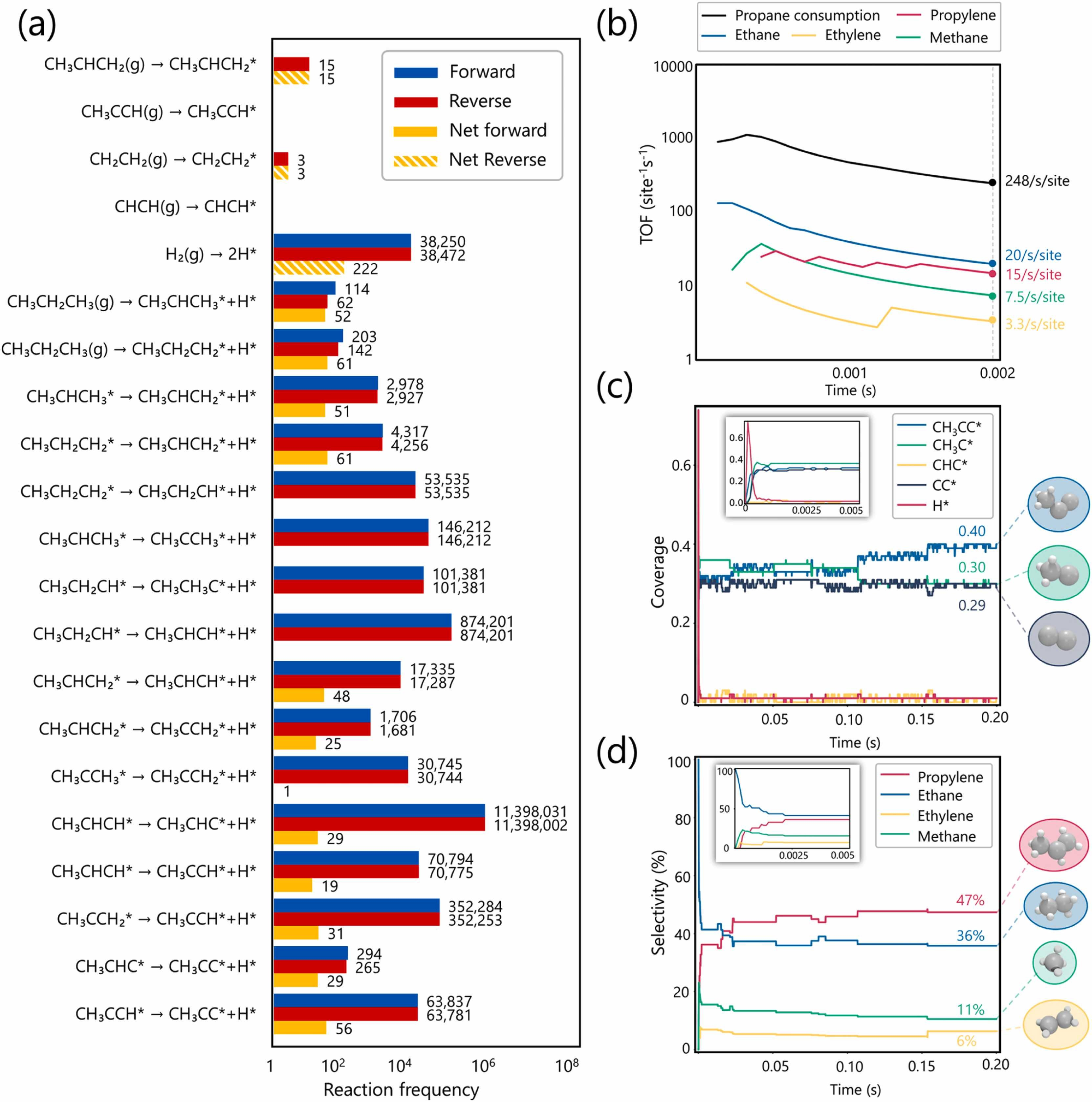
미시동역학: TOF + 피복률 + 선택성

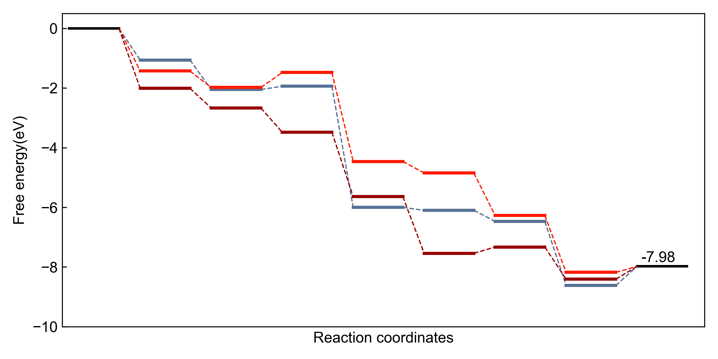
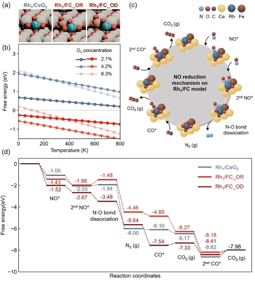
반응 좌표 다이어그램

1

왜 Python인가?

LLM 시대의 자동화

1.1

왜 Python인가 & 좋은 그래프란?

왜 Python인가?

자동화: 두 번 하면 자동화하라
LLM 시대는 완전한 자동화를 가능하게 함
코드 기반 = 재현 가능 & 버전 관리
반복 작업이 아닌 연구에 집중

좋은 그래프의 조건...

심미성: 색상 조화, 시각적 매력
명료성: 명확한 연구 메시지
관례: 분야 표준 준수
원칙: 하나의 색/모양 = 하나의 의미

->

Python + LLM = 효율적이고 재현 가능하며 아름다운 그래프

1.2

예시: 에너지 다이어그램 & 전기화학

구조 + 열역학 + 에너지 다이어그램

다중 경로 반응 좌표

분극 곡선 (j vs E)

볼케이노 플롯 + 메커니즘 + 전하 밀도

2

Python 기초

환경 설정, Matplotlib, 데이터 처리

2.1

환경 설정 & 임포트

Conda 설정

# 환경 생성
conda create -n mpl python=3.9
conda activate mpl

# 패키지 설치
conda install matplotlib pandas numpy
pip install ase  # 선택사항

기본 임포트

import matplotlib.pyplot as plt
import numpy as np
import pandas as pd

# 사용자 정의 폰트용
import matplotlib.font_manager as fm

IDE 옵션

VSCode / Cursor (AI 지원)
Google Colab

핵심 라이브러리

matplotlib: 그래프 작성
numpy: 배열
pandas: 데이터 I/O

2.2

Figure, Axes & 플롯 유형

fig, ax 패턴 (권장)

fig, ax = plt.subplots(figsize=(8, 6))
ax.plot(x, y, color='blue', lw=2)

# 다중 서브플롯
fig, axes = plt.subplots(2, 3)
axes[0, 0].plot(x, y)

플롯 유형

# 선 플롯
ax.plot(x, y, 'b-', label='data')

# 산점도
ax.scatter(x, y, s=50, alpha=0.7)

# 영역 채우기
ax.fill_between(x, y1, y2, alpha=0.3)

항상 fig, ax 패턴을 사용하세요. 원시 데이터는 scatter, 연속/처리된 데이터는 line을 사용합니다.

2.3

레이블, 범위, 범례 & 저장

포매팅

# 레이블과 범위
ax.set_xlabel('온도 (C)')
ax.set_ylabel('전환율 (%)')
ax.set_xlim(0, 100)
ax.set_ylim(0, 100)

# 범례
ax.legend(loc='upper right')

저장

# 항상 먼저 tight_layout!
plt.tight_layout()

# 옵션과 함께 저장
plt.savefig('fig.png', dpi=300,
            bbox_inches='tight')
plt.savefig('fig.svg')  # 벡터

SVG 형식이 출판물에 가장 적합 (벡터, 확장 가능)

인쇄 품질을 위해 최소 dpi=300

XPS 축 반전: ax.set_xlim(x.max(), x.min())

2.4

데이터 처리: NumPy & Pandas

NumPy 배열

# 벡터화 연산 (빠름!)
data = np.array([1, 2, 3, 4, 5])
squared = data**2  # 한 번에 모두

# 배열 생성
x = np.linspace(0, 10, 100)
x = np.arange(0, 10, 0.1)
y = np.sin(x)

Pandas로 Excel/CSV 읽기

df = pd.read_excel('data.xlsx',
                   sheet_name='Sheet1')

# 열 선택
x = df.iloc[:, 0]  # 위치로
y = df['col_name']  # 이름으로

# 데이터 정리
df = df.dropna()  # NaN 제거

.values를 사용하여 pandas Series를 플로팅용 numpy 배열로 변환하세요.

3

LLM 가속화

AI 기반 그래프 생성

3.1

LLM 도구 & 시스템 프롬프트

💬

챗봇

아이디어 발상, 빠른 코드 스니펫에 적합

✎

Cursor

미세 조정, 에디터 내 AI

💻

Claude Code

완전 자동화, 바이브 코딩

🚀

Copilot

코드 자동완성

# 일관된 그래프를 위한 시스템 프롬프트
fs = 12  # 폰트 크기
font_props = fm.FontProperties(family='Arial', size=fs)
colors = ['#77AEB3', '#E5885D', '#C7C4B5', '#A1C2DE', '#B4944B']
os.makedirs('./output', exist_ok=True)

3.2

헬퍼 함수 & 완성 예제

def format_axis(ax, xlabel, ylabel):
    ax.set_xlabel(xlabel, fontproperties=font_props)
    ax.set_ylabel(ylabel, fontproperties=font_props)

def save_plot(filename):
    plt.tight_layout()
    plt.savefig(f'./output/{filename}', dpi=300, bbox_inches='tight')

# 완성 예제
x = np.linspace(0, 10, 100)
fig, ax = plt.subplots(figsize=(8, 6))
ax.plot(x, np.sin(x), 'b-', lw=2, label='sin(x)')
ax.plot(x, np.cos(x), 'r--', lw=2, label='cos(x)')
ax.fill_between(x, np.sin(x), np.cos(x), where=(np.sin(x)>np.cos(x)), alpha=0.3)
format_axis(ax, 'X 값', 'Y 값')
ax.legend()
save_plot('trig.svg')

3.3

핵심 요약

1fig, ax 패턴 사용

2단위와 함께 레이블 설정

3저장 전 tight_layout()

4bbox_inches='tight'

5레이어에 alpha 사용

6출판물에는 SVG

1

NumPy + Pandas

속도를 위한 배열, Excel/CSV용 DataFrame

2

Matplotlib

fig/ax 패턴, 일관된 스타일링, 올바른 저장

3

LLM 도구

미세 조정에 Cursor, 자동화에 Claude Code

아름다운 그래프는 이야기를 전합니다

자동화, 반복, 완성

좋은 그래프는 연습이 필요합니다

자동화는 창의성을 위한 시간을 절약합니다

LLM은 당신의 코딩 파트너입니다

계속 코딩하세요. 계속 시각화하세요. 계속 출판하세요.